── Conflicts ────────────────────────────────────────── tidyverse_conflicts() ──
✖ psych::%+%()        masks ggplot2::%+%()
✖ psych::alpha()      masks ggplot2::alpha(), scales::alpha()
✖ readr::col_factor() masks scales::col_factor()
✖ purrr::discard()    masks scales::discard()
✖ dplyr::filter()     masks stats::filter()
✖ stringr::fixed()    masks recipes::fixed()
✖ dplyr::lag()        masks stats::lag()
✖ readr::spec()       masks yardstick::spec()
ℹ Use the conflicted package (<http://conflicted.r-lib.org/>) to force all conflicts to become errors
library(corrplot) # creating correlation plots
corrplot 0.92 loaded
Next, I will read the csv file to import the Mavoglurant data into R.
trial_data <-read_csv(here("fitting-exercise", "Mavoglurant_A2121_nmpk.csv"), show_col_types =FALSE) # read csv in the relative path to the fitting exercise folder, without showing column typesstr(trial_data) # examine structure of data in the trial_data frame
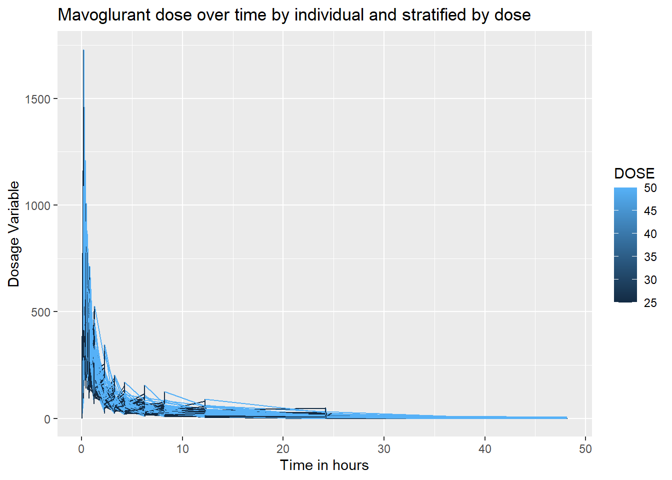
I want to create a line plot showing a dosage over time for each individual in the data set, that is stratified by total dose amount.
ggplot(trial_data, aes(x = TIME, y = DV, group = ID, color = DOSE)) +geom_line() +labs(title ="Mavoglurant dose over time by individual and stratified by dose", y="Dosage Variable", x ="Time in hours")
Because the value of 2 for OCC (or occasion) reflects 2 dosages, and we are only examining cases that are given 1 dose, we will drop all levels= ‘2’ of the factor variable, OCC.
trial_data <-droplevels(trial_data[!trial_data$OCC =='2',]) # drop rows where the level value is '2'str(trial_data) # examine dataframe structure
levels(trial_data$OCC) # examine levels of the OCC variable
[1] "1"
All factor levels of OCC except for ‘1’, were dropped. Next, we will drop all rows with the numeric value for TIME = ‘0’
trial_data2 <-trial_data[!(trial_data$TIME %in%0),] # exclude all rows where time has a value fo zerosummary(trial_data2$TIME) # check the minimum avlue for TIME
   Min. 1st Qu.  Median    Mean 3rd Qu.    Max.
  0.200   0.583   3.200   6.930   8.250  48.217
Now we will use dplyr to find the sum of dosage values (DV) for each individual (ID).
sum_DV <- trial_data2 %>%# create data frame for the sum_DVgroup_by(ID) %>%# group by individual summarise( Y =sum(DV)) # make a summary column of DV using dpylrstr(sum_DV) # check structure of sumDV
trial_data4 <-merge(x = trial_data3, y = sum_DV, by ="ID", all =TRUE) # outer join the data frame to preserve all rows and join them by the ID variablestr(trial_data4) # check structure of joined df
Because I have already converted the variables, SEX and RACE, to factors, I will not repeat this step. I will delete the unnecessary columns of my final data frame to only include the variables: Y, DOSE, AGE, SEX, RACE, WT, and HT.
trial_data4 <- trial_data4 %>%select("Y", "DOSE", "AGE", "SEX", "RACE", "WT", "HT") # select only the aforementioned variablesstr(trial_data4) # check data structure
       Y               DOSE            AGE        SEX     RACE
 Min.   : 826.4   Min.   :25.00   Min.   :18.00   1:104   1 :74
 1st Qu.:1700.5   1st Qu.:25.00   1st Qu.:26.00   2: 16   2 :36
 Median :2349.1   Median :37.50   Median :31.00           7 : 2
 Mean   :2445.4   Mean   :36.46   Mean   :33.00           88: 8
 3rd Qu.:3050.2   3rd Qu.:50.00   3rd Qu.:40.25
 Max.   :5606.6   Max.   :50.00   Max.   :50.00
       WT               HT
 Min.   : 56.60   Min.   :1.520
 1st Qu.: 73.17   1st Qu.:1.700
 Median : 82.10   Median :1.770
 Mean   : 82.55   Mean   :1.759
 3rd Qu.: 90.10   3rd Qu.:1.813
 Max.   :115.30   Max.   :1.930
I will now check for any missing values.
which(is.na(trial_data4)) # find location of missing values
integer(0)
sum(is.na(trial_data4)) # count total missing values
[1] 0
path <-here("./fitting-exercise/cleandata.rds") # create path using here packagesaveRDS(trial_data4, file = path) # save as an rds using specified here path
No missing variables will found, so I will not continue to clean the data and move onto exploratory data analysis. I save the clean data as an rds called cleandata.rds. ## Exploratory Data Analysis ### Summary Table I will create a summary table of the data frame in R by using the describe() function from the “psych” package.
table1 <-describe(trial_data4[ , c("Y", "DOSE", "AGE","WT", "HT")],fast=TRUE) # summary stats of cleaned data for the numeric columnsprint(table1)
     vars   n    mean     sd    min     max   range    se
Y       1 120 2445.41 961.64 826.43 5606.58 4780.15 87.78
DOSE    2 120   36.46  11.86  25.00   50.00   25.00  1.08
AGE     3 120   33.00   8.98  18.00   50.00   32.00  0.82
WT      4 120   82.55  12.52  56.60  115.30   58.70  1.14
HT      5 120    1.76   0.09   1.52    1.93    0.41  0.01
In this summary table, we see the numeric variables. They all have a relatively small SE and reasonable min and max values. The range sumDV (Y) is large, but this is likely because this is the sum of the concentration administered to each individual. Now I will bring in the factor variables. I want to stratify the Y variable and dose by AGE, RACE, AGE, WT and HT. I will be using the tidyverse and gtsummary (which I found on stackoverflow) packages to produce this table.
`summarise()` has grouped output by 'SEX'. You can override using the `.groups`
argument.
print(table2)
# A tibble: 8 × 8
# Groups:   SEX [2]
  SEX   RACE  mean_Y mean_DOSE mean_AGE  sd_Y sd_DOSE sd_AGE
  <fct> <fct>  <dbl>     <dbl>    <dbl> <dbl>   <dbl>  <dbl>
1 1     1      2468.      38.1     32.9  995.    11.8   9.14
2 1     2      2497.      35.6     31.0  910.    12.2   7.91
3 1     7      1491.      25       41     NA     NA    NA
4 1     88     2612.      35.7     24.6  974.    13.4   3.64
5 2     1      2239.      34.1     40.7 1099.    11.3   6.08
6 2     2      2087.      25       39   1010.     0    10.1
7 2     7      2790.      50       49     NA     NA    NA
8 2     88     2093.      25       39     NA     NA    NA
The means of Y and dosage seam to be similar, and within the range specified above with a couple exceptions. SEX(1) and RACE(7) has a lower mean Y. There is also a high DOSE value for SEX(2) RACE(7). This value of 50 is the max, so either all of the values here must be 50. The mean age for race and sex also varies quite a bit. It is also strange the sd for dose for SEX(2) RACE(2) is 0. ### Data Distribution #### Scatter Plots To examine these strange summary stats in the table in more detail, we will visualize the data distribution using ggplot2. First, I will produce some scatterplots to see if there are any associations or if the data is randomly distributed
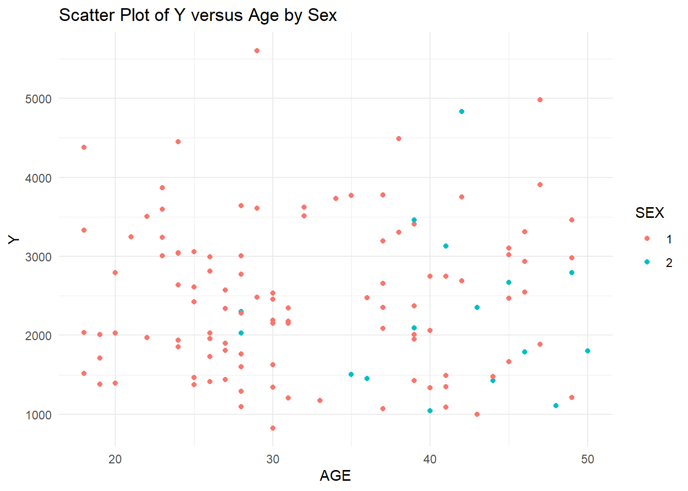
# Y versus AGE scatter plot by SEXplot1 <-ggplot(trial_data4, aes(x = AGE, y = Y, color = SEX)) +geom_point() +labs(x ="AGE", y ="Y", title ="Scatter Plot of Y versus Age by Sex") +theme_minimal()print(plot1)
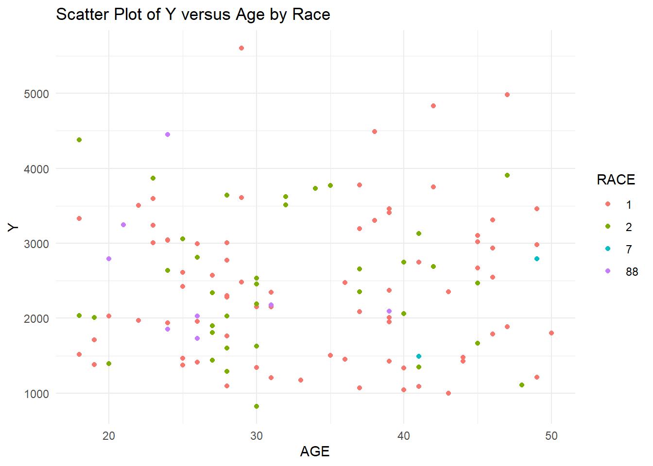
# Y versus AGE scatter plot by RACEplot2 <-ggplot(trial_data4, aes(x = AGE, y = Y, color = RACE)) +geom_point() +labs(x ="AGE", y ="Y", title ="Scatter Plot of Y versus Age by Race") +theme_minimal()print(plot2)
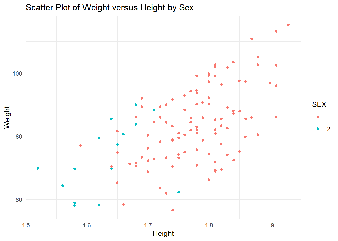
# WT versus HT scatter plot by Sexplot3 <-ggplot(trial_data4, aes(x = HT, y = WT, color = SEX)) +geom_point() +labs(x ="Height", y ="Weight", title ="Scatter Plot of Weight versus Height by Sex") +theme_minimal()print(plot3)
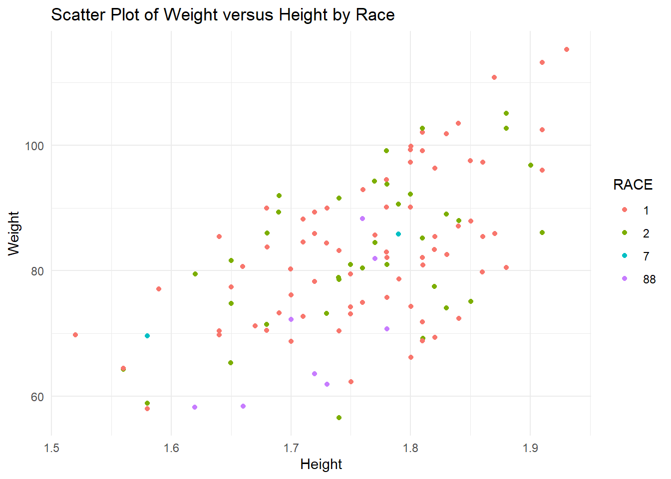
# WT versus HT scatter plot by Raceplot4 <-ggplot(trial_data4, aes(x = HT, y = WT, color = RACE)) +geom_point() +labs(x ="Height", y ="Weight", title ="Scatter Plot of Weight versus Height by Race") +theme_minimal()print(plot4)
The distribution of age seems and Y seem to be fairly random, with the exception of an outlier in the Y variable that is extremely high. I will leave this outlier as there is no indication of whether this holds importance (we don’t know the definition of many of these variables). The distribution of Sex for Y and Age values seems to be a higher age for sex 2, but random for the Y variable. In general, Race seems fairly random for Age and Y, except Race 7 seems to also predominantly be higher ages. Weight and height show a slight trend, as they normally do, without any extreme outliers. The sex distribution of height and weight also makes sense as females tend to be shorter and weight less than males. For this reason, we might assume that sex 2 is female, but we should not make assumptions. Races 1, 2, and 7 seem to be randomly distributed for weight and height. However, race 88 seems to be on the lower end for both height and weight, which may indicate some sex correlation with race. #### Box Plots Now I will use box plots to examine the distribution of Dose and Y stratified by the two factor variables, Race and Sex.
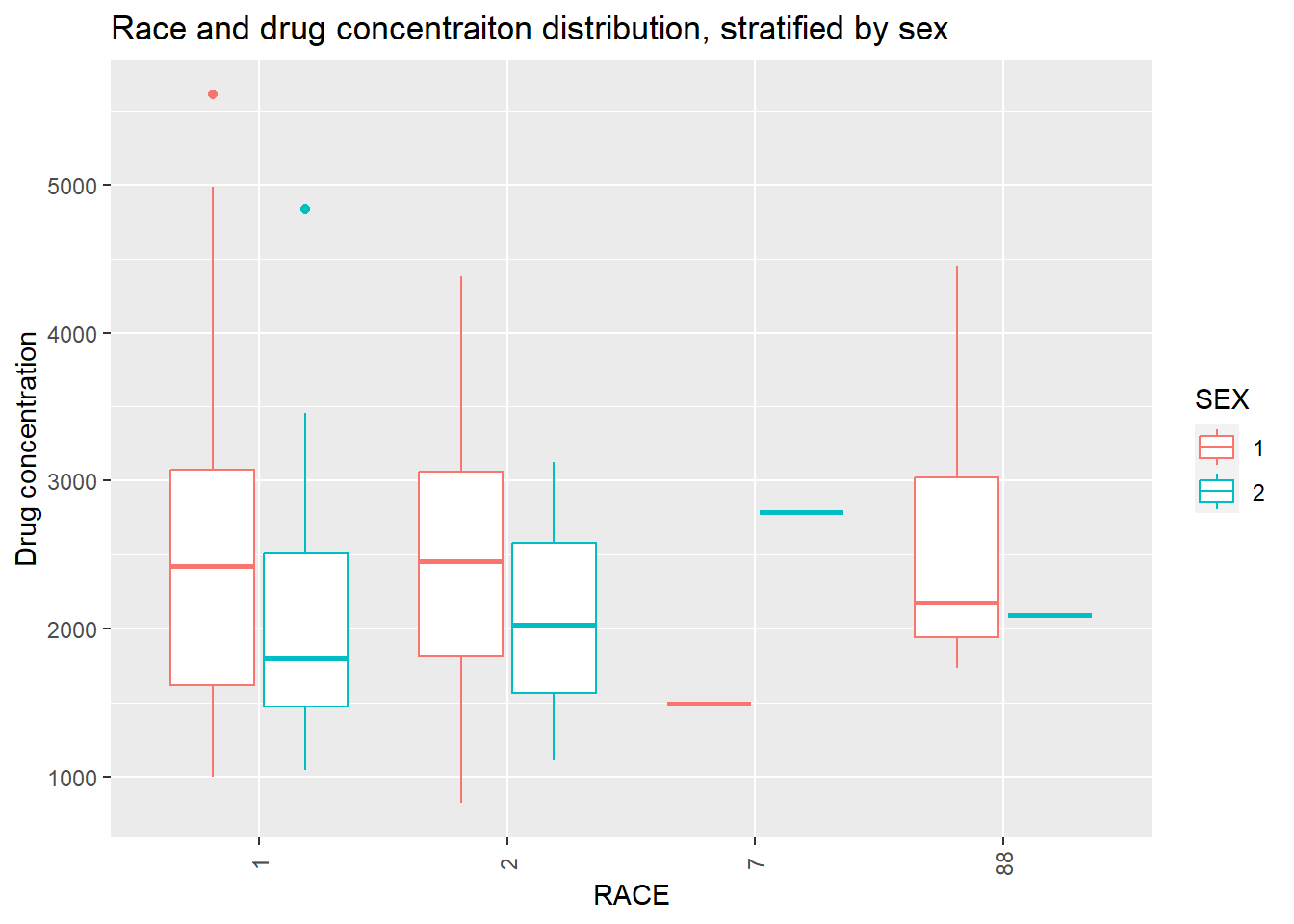
# Distribution of Y stratified by SEX and RACEplot6 <- trial_data4 %>%ggplot(aes(x=RACE, y=Y, color = SEX)) +geom_boxplot() +labs(x ="RACE", y ="Drug concentration", title ="Race and drug concentraiton distribution, stratified by sex") +theme(axis.text.x =element_text(angle =90, vjust =0.5)) # Rotate x-axis text by 90 degreesplot(plot6)
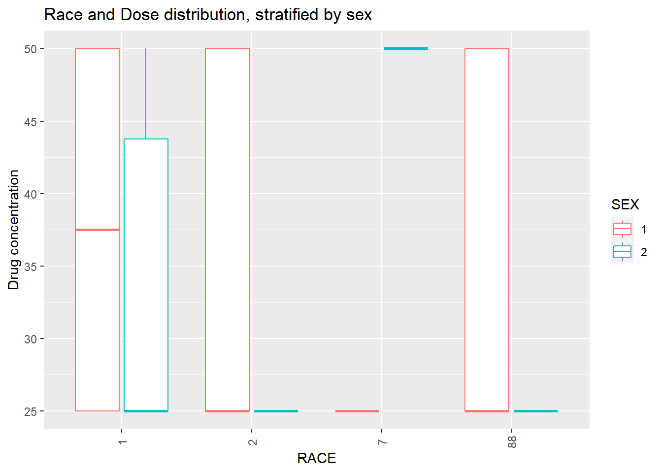
# Distribution of DOSE stratified by SEX and RACEplot7 <- trial_data4 %>%ggplot(aes(x=RACE, y=DOSE, color = SEX)) +geom_boxplot() +labs(x ="RACE", y ="Drug concentration", title ="Race and Dose distribution, stratified by sex") +theme(axis.text.x =element_text(angle =90, vjust =0.5)) # Rotate x-axis text by 90 degreesplot(plot7)
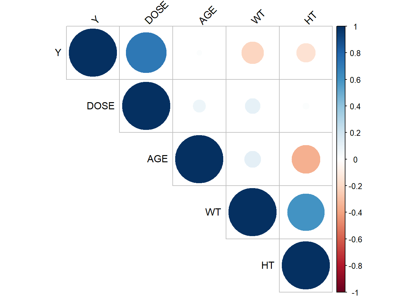
There are two outliers for Y, in race 1. Each outlier is of a different sex, so sex might not impact the outliers.There are only 2 values for race 7, making their distribution look wonky. In general, sex 1 has a higher Y and dose than sex 2. No outliers is dose were seen as there are only 3 options for dose. Again, because there are two values in race 7, the distribution is wonky. I will choose to keep Race 7, because I do not know if this represents an important minority group, despite there only being 2 values. ### Correlation Plots Now I will create a correlation plot of the numeric variables. To do this, I asked ChatGPT to provide me with the functions used to make correlation plots for numeric variables.
From the correlation plot, it seems that weight and height, and Y and Dose are most highly correlated. Age and height are moderately negatively correlated, as well as weight and Y are slightly negatively correlated. ## Model Fitting First, I will fit a linear model to the outcome, Y, using the predictor of DOSE.
set.seed(333)data_split <- trial_data4 %>%initial_split(prop =3/4) #split the data so that 3/4 is in the training set and 1/4 in the reference settrain_data <-training(data_split) # make the training data objecttest_data <-testing(data_split) # make testing data objecttrial_linear_fit_1 <-recipe(Y ~ DOSE, data = train_data) lm_mod <-linear_reg() %>%# make object called lm_mod for linear_regression functionset_engine("lm") %>%# set linear regression engine to lmset_mode("regression") # set to regression modetrials_workflow1 <-workflow() %>%#create a workflowadd_model(lm_mod) %>%#apply the linear regression modeladd_recipe(trial_linear_fit_1) #then, apply the recipelm_fit <- lm_mod %>%fit(Y ~ DOSE, data = trial_data4) # fit Y to dose tidy(lm_fit) # produce tibble for linear regression fit
The intercept has a relatively large standard error, while the DOSE regression estimate has a more reasonable SE. This linear regression reflects a positive trend between dose and Y with a slope of 58.2. I will now use this model to predict the trial data. This will allow me to calculate the predictive power using the RMSE and R-squared metrics.
trial_fit1 <- trials_workflow1 %>%fit(data = train_data) # shows model to fit the data used from training from the aforementioned workflowpredict(trial_fit1, test_data) #predict the outcome Y
eval_metrics <-metric_set(rmse, rsq) # use yardstick to select multiple regression metrics (rmse and r squared)eval_metrics(data = trial_aug,truth = Y,estimate = .pred) %>%select(-2) # Evaluate RMSE, R2 based on the results
The RMSE is very large and rsq is close to 0.5 which shows that the predictive model is not a very good fit for the data. Next, I will fit a linear model to the outcome, Y, using all of the predictors.
trial_linear_fit_2 <-recipe(Y ~ ., data = train_data) lm_mod2 <-linear_reg() %>%# make object called lm_mod for linear_regression functionset_engine("lm") %>%# set linear regression engine to lmset_mode("regression") # set to regression modetrials_workflow2 <-workflow() %>%#create a workflowadd_model(lm_mod2) %>%#apply the linear regression modeladd_recipe(trial_linear_fit_2) #then, apply the recipelm_fit2 <- lm_mod2 %>%fit(Y ~ ., data = trial_data4) # fit Y to dose tidy(lm_fit2) # produce tibble for linear regression fit
The standard error for the intercept, SEX2, RACE2, Race7, and HT are extremely large. This may be in part due to the large standard error of the original Y (outcome) variable. Dose, Age and Race2 have a positive trend with Y while the variables Sex2, Race7, Race88, WT, and HT have a negative trend with Y.
trial_fit2 <- trials_workflow2 %>%fit(data = train_data) # shows model to fit the data sued from training from the aforementioned workflowpredict(trial_fit2, test_data) #predict the outcome Y
eval_metrics <-metric_set(rmse, rsq) # use yardstick to select multiple regression metrics (rmse and r squared)eval_metrics(data = trial_aug,truth = Y,estimate = .pred) %>%select(-2) # Evaluate RMSE, R2 based on the results
The R squared value for the model including all of the predictors is slightly better than the previous model (at around 0.6), but still NOT good. The rmse has not changed much, reflecting a large impact of outliers on the standard error of the predictions in the linear model.
Now we will make a model with SEX to practice fitting with a categorical outcome variable. We will fit a logistic model to the SEX outcome using the predictor, DOSE.
trial_logreg_rec <-recipe(SEX ~ DOSE, data = train_data) %>%# create recipe for logistic regression model using SEX as outcomeprep() # Prepare the recipelr_mod <-logistic_reg() %>%# make object called lr_mod for logistic regression functionset_engine("glm") # set logistic regression engine to glmlr_trials_workflow <-workflow() %>%# create a workflowadd_model(lr_mod) %>%# apply the logistic regression modeladd_recipe(trial_logreg_rec) # then, apply the recipelr_fit <- lr_mod %>%fit(SEX ~ DOSE, data = trial_data4) # fit Y to dose tidy(lr_fit) # produce tibble for log regression fit
There is a relatively high standard error for both the dose and intercept estimates. Both estimates are negative, meaning there is a negative trend between dose and sex.
We will now compute accuracy and ROC-AUC for this model.
The AUC metric for the first predictor is 0.62 and for the second is 0.38. They are both the same magnitude away from 0.5. This means that both predictions are equally as good, but neither prediction is great because it they are not very close to 1 or 0. This means that this model doesn’t have great predictive power either.
Next, we will fit a logistic model to SEX using all of the other predictors.
trial_logreg_rec2 <-recipe(SEX ~ ., data = train_data) %>%# create recipe for logistic regression model using SEX as outcomeprep() # Prepare the recipelr_mod2 <-logistic_reg() %>%# make object called lr_mod for logistic regression functionset_engine("glm") # set logistic regression engine to glmlr_trials_workflow2 <-workflow() %>%# create a workflowadd_model(lr_mod2) %>%# apply the logistic regression modeladd_recipe(trial_logreg_rec2) # then, apply the recipelr_fit2 <- lr_mod2 %>%fit(SEX ~ ., data = trial_data4) # fit Y to dose tidy(lr_fit2) # produce tibble for log regression fit
The intercept now has a much higher estimate, of 60 and a smaller SE than the previous logistic regression model. Almost all of the variables have a negative trends with the Sex variables, except for Race7. In addition, all of the estimates for the predictor variables versus Sex (outcome) have a very high SE, meaning that they have a high variability.
We will also compute accuracy and ROC-AUC for this model.
With a AUC of 0.62 and 0.38, both predictions are equally good, but also both not the greatest. AUC values closer to 0.5 means the model is more near a random model versus an AUC close to 0 or 1, which might show good predictive power.
Part 2
Model Improvement
For this exercise, we will be using the data previously used to fit our linear and logistic models to create new models and improve those models. We will be using tidymodels and the packages previously opened for the first part of this exercise. We will start this exercise by eliminating the variable entitled RACE because it has values (7 and 88) with too few observations, and which might be acting as outliers.
trial_data5 <-subset(trial_data4, select =-RACE) # Use subset to column to drop str(trial_data5) # check structure of new df
'data.frame':   120 obs. of  6 variables:
 $ Y   : num  2691 2639 2150 1789 3126 ...
 $ DOSE: num  25 25 25 25 25 25 25 25 25 25 ...
 $ AGE : num  42 24 31 46 41 27 23 20 23 28 ...
 $ SEX : Factor w/ 2 levels "1","2": 1 1 1 2 2 1 1 1 1 1 ...
 $ WT  : num  94.3 80.4 71.8 77.4 64.3 ...
 $ HT  : num  1.77 1.76 1.81 1.65 1.56 ...
Next, we will set a seed for reproducibility. And split the data with 75% in the training set and 25% in the testing set.
rngseed <-1234set.seed(rngseed) # set seed according to the variable rngseed (which equals 1234)# Data Splittinglibrary(rsample)trial5_split <-initial_split(trial_data5, prop =3/4)# create new data frame with the 3/4 splittrain_data2 <-training(trial5_split) # create data frame for training datatest_data2 <-testing(trial5_split) # create data frame for testing data
Next, I will produce a linear model with just one predictor, DOSE, the outcome, or the Y variable. I will then produce a full model including all of the predictors: DOSE, AGE, SEX, WT, and HT.
# Single Predictor Model (Y v. DOSE)single_rec <-recipe(Y ~ DOSE, data = train_data2) # specify the recipe by putting the formula for the null linear modelsingle_linreg <-linear_reg() %>%# make object called null_linreg for linear_regression functionset_engine("lm") %>%# set linear regression engine to lmset_mode("regression") # set to regression modeworkflow_single <-workflow() %>%#create a workflow for the linear model called workflow_nulladd_model(single_linreg) %>%#apply the linear regression modeladd_recipe(single_rec) #then, apply the recipesingle_lmfit <- workflow_single %>%fit(data = train_data2) # fit Y to dose using ONLY the training datatidy(single_lmfit) # produce tibble for linear regression fit
# Full model (Y v. all predictors)full_rec <-recipe(Y ~ ., data = train_data2) # specify the recipe by putting the formula for the linear model with all the predictorsfull_linreg <-linear_reg() %>%# make object called full_linreg for linear_regression functionset_engine("lm") %>%# Use the same linear regression engine as the null modelset_mode("regression") # and also, set to regression modeworkflow_full <-workflow() %>%#create a workflow for the full linear model called workflow_fulladd_model(full_linreg) %>%#apply the new linear regression modeladd_recipe(full_rec) #then, apply the recipefull_lmfit <- workflow_full %>%# add the workflow to the fitfit(data = train_data2) # fit Y to dose using ONLY the training datatidy(full_lmfit) # produce tibble to organize the resulting linear regression fit
Now I will compute the predictions that are made by both the singular predictor model and the full model. RMSE will be calculated using the observed versus the predicted values. Lastly, we will compare these RMSE values to the RMSE of the null model as fitted using the null_model() function.
#Edited by Taylor Glass I noticed that the reason your RMSE values were not as expected is because you were using the test_data2 instead of the train_data2. This entire process should be using the train_data2 only, so I made those changes. The RMSE values are now 948, 702, and 627 respectively.
# Make predictions with the single predictor linear modelpredict(single_lmfit, train_data2) #predict the outcome Y from the single predictor linear model (Y v. dose)
single_aug <-augment(single_lmfit, train_data2) # add columns of interest to new data framesingle_aug %>%select("Y", "DOSE") # select columns to add to the data frame
# Calculate the RMSE of the single predictor modelrmse_sing <-rmse(data = single_aug,truth = Y,estimate = .pred)print(rmse_sing) # Evaluate RMSE based on the results
# A tibble: 1 × 3
  .metric .estimator .estimate
  <chr>   <chr>          <dbl>
1 rmse    standard        703.
# Make predictions with the full predictor linear modelpredict(full_lmfit, train_data2) #predict the outcome Y from the FULL predictor linear model (Y v. all predictors)
full_aug <-augment(full_lmfit, train_data2) # add predictions to new data framefull_aug %>%select("Y", "DOSE", "AGE", "SEX", "WT", "HT") # select columns to add to the data frame
# Calculate the RMSE of the full modelrmse_full <-rmse(data = full_aug,truth = Y,estimate = .pred)print(rmse_full) # Evaluate RMSE based on the results
# A tibble: 1 × 3
  .metric .estimator .estimate
  <chr>   <chr>          <dbl>
1 rmse    standard        627.
# Make predictions using a null modelblank_model <-null_model() %>%set_engine("parsnip") %>%set_mode("regression") # use the null_model function and the parsnip engine to create a blank modelblank_rec <-recipe(Y ~1, data = train_data2) # produce recipe for blank modelworkflow_blank <-workflow() %>%#create a workflow for the null model called workflow_blankadd_model(blank_model) %>%#apply the new null modeladd_recipe(blank_rec) #then, apply the recipeblank_fit <- workflow_blank %>%# add the workflow to the fitfit(data = train_data2) # fit Y to dose using ONLY the training datatidy(blank_fit) # produce tibble to organize the resulting linear regression fit
# A tibble: 1 × 1
  value
  <dbl>
1 2509.
predict(blank_fit, train_data2) #predict the outcome Y from the BLANK predictor linear model
blank_aug <-augment(blank_fit, train_data2) # add predictions to new data frameblank_aug %>%select("Y", "DOSE", "AGE", "SEX", "WT", "HT") # select columns to add to the data frame
names(blank_aug) # check the names for the columns
[1] "Y" "DOSE" "AGE" "SEX" "WT" "HT" ".pred"
# Calculate the RMSE of the blank modelrmse_blank <-rmse(data = blank_aug,truth = Y,estimate = .pred)print(rmse_blank) # Evaluate RMSE based on the results
# A tibble: 1 × 3
  .metric .estimator .estimate
  <chr>   <chr>          <dbl>
1 rmse    standard        948.
The RMSE for the single predictor model, full model, and null model are 560, 520, and 993 respectively. This is not equal to the values found by Dr. Handel, however I did set the seed in the initial step. The RMSE of both the full and single predictor models are similar, with a difference of 60, while the RMSE for the null model is much greater than both models including predictors. The null model has an RMSE that with a difference of 433 and 393 for the single predictor and full models, respectively. This reflects that both models that contain predictors are better at predicting values based on the original observations, than the null model is at predicting the observations. This means that both models including predictors are better than random models, and capture some trend using linear regression. ### Using cross validation to evaluate linear models I will now use cross validation to evaluate the linear models and null model that were produced. Cross validation is a re-sampling method to measure model performance while accounting for the variance-bias trade off. Here, we will use a 10-fold cross validation method, which compares the train and test data 10 times (using different subsamples) using RMSE to check for consistancy in model predictions. I start by specifying the workflow for the cross validation method. Then I will use the fit_resamples function to perform the CV fit. I will use RMSE to compare each models’ CV fit.
# Single Predictor Linear Model Cross Validationfolds <-vfold_cv(trial_data5, v =10)single_cv_wf <-workflow() %>%#define an object for the cv workflow add_model(single_linreg) %>%# add in the previous linear modeladd_recipe(single_rec) # specify the formula for the first linear modelsingle_fit_cv <- single_cv_wf %>%# apply cv workflow to an object for the cv fitfit_resamples(folds) # specify the number of folds for the cvprint(single_fit_cv)
# Examine rmse of the cv fitrmse_values1 <- single_fit_cv %>%collect_metrics() %>%# get the metrics for all of the re-sampled foldsfilter(.metric =="rmse") # filter by the rmse values onlyprint(rmse_values1)
# A tibble: 1 × 6
  .metric .estimator  mean     n std_err .config
  <chr>   <chr>      <dbl> <int>   <dbl> <chr>
1 rmse    standard    663.    10    52.6 Preprocessor1_Model1
# Full Linear Model Cross Validationfull_cv_wf <-workflow() %>%#define an object for the cv workflow add_model(full_linreg) %>%# add in the previous linear modeladd_recipe(full_rec) # specify the formula for the first linear modelfull_fit_cv <- full_cv_wf %>%# apply cv workflow to an object for the cv fitfit_resamples(folds) # specify the number of folds for the cv# Examine rmse of the cv fitrmse_values2 <- full_fit_cv %>%collect_metrics() %>%# get the metrics for all of the re-sampled foldsfilter(.metric =="rmse") # filter by the rmse values onlyprint(rmse_values2)
# A tibble: 1 × 6
  .metric .estimator  mean     n std_err .config
  <chr>   <chr>      <dbl> <int>   <dbl> <chr>
1 rmse    standard    619.    10    46.7 Preprocessor1_Model1
# Null Model Cross Validationnull_cv_wf <-workflow() %>%#define an object for the cv workflow add_model(blank_model) %>%# add blank model inadd_recipe(blank_rec)null_fit_cv <- null_cv_wf %>%# apply cv workflow to an object for the cv fitfit_resamples(folds) # specify the number of folds for the cv
→ A | warning: A correlation computation is required, but `estimate` is constant and has 0 standard deviation, resulting in a divide by 0 error. `NA` will be returned.
There were issues with some computations A: x1
There were issues with some computations A: x10
# Examine rmse of the cv fitrmse_values3 <- null_fit_cv %>%collect_metrics() %>%# get the metrics for all of the re-sampled foldsfilter(.metric =="rmse") # filter by the rmse values onlyprint(rmse_values3)
# A tibble: 1 × 6
  .metric .estimator  mean     n std_err .config
  <chr>   <chr>      <dbl> <int>   <dbl> <chr>
1 rmse    standard    948.    10    63.7 Preprocessor1_Model1
The mean RMSE for both models including predictors greatly increased, while the mean RMSE for the null model stayed nearly the same. For the model including a single predictor, the RMSE increased by 99 and the full model RMSE increased by 97. Both models had an rmse value increase by approximately the same magnitude. The standard error for all three models (including the null) are very similar (58, 53, and 55), which demonstrates consistency between models despite varying numbers of predictors being used.
Lastly, I will run the code again with a different seed to see if the cross validation and rmse values change.
set.seed(333)# Single Predictor Linear Model Cross Validationfolds <-vfold_cv(trial_data5, v =10)single_cv_wf <-workflow() %>%#define an object for the cv workflow add_model(single_linreg) %>%# add in the previous linear modeladd_recipe(single_rec) # specify the formula for the first linear modelsingle_fit_cv <- single_cv_wf %>%# apply cv workflow to an object for the cv fitfit_resamples(folds) # specify the number of folds for the cvprint(single_fit_cv)
# Examine rmse of the cv fitrmse_values1 <- single_fit_cv %>%collect_metrics() %>%# get the metrics for all of the re-sampled foldsfilter(.metric =="rmse") # filter by the rmse values onlyprint(rmse_values1)
# A tibble: 1 × 6
  .metric .estimator  mean     n std_err .config
  <chr>   <chr>      <dbl> <int>   <dbl> <chr>
1 rmse    standard    669.    10    28.3 Preprocessor1_Model1
# Full Linear Model Cross Validationfull_cv_wf <-workflow() %>%#define an object for the cv workflow add_model(full_linreg) %>%# add in the previous linear modeladd_recipe(full_rec) # specify the formula for the first linear modelfull_fit_cv <- full_cv_wf %>%# apply cv workflow to an object for the cv fitfit_resamples(folds) # specify the number of folds for the cv# Examine rmse of the cv fitrmse_values2 <- full_fit_cv %>%collect_metrics() %>%# get the metrics for all of the re-sampled foldsfilter(.metric =="rmse") # filter by the rmse values onlyprint(rmse_values2)
# A tibble: 1 × 6
  .metric .estimator  mean     n std_err .config
  <chr>   <chr>      <dbl> <int>   <dbl> <chr>
1 rmse    standard    606.    10    47.7 Preprocessor1_Model1
# Null Model Cross Validationnull_cv_wf <-workflow() %>%#define an object for the cv workflow add_model(blank_model) %>%# add blank model inadd_recipe(blank_rec)null_fit_cv <- null_cv_wf %>%# apply cv workflow to an object for the cv fitfit_resamples(folds) # specify the number of folds for the cv
→ A | warning: A correlation computation is required, but `estimate` is constant and has 0 standard deviation, resulting in a divide by 0 error. `NA` will be returned.
There were issues with some computations A: x1
There were issues with some computations A: x7
There were issues with some computations A: x10
# Examine rmse of the cv fitrmse_values3 <- null_fit_cv %>%collect_metrics() %>%# get the metrics for all of the re-sampled foldsfilter(.metric =="rmse") # filter by the rmse values onlyprint(rmse_values3)
# A tibble: 1 × 6
  .metric .estimator  mean     n std_err .config
  <chr>   <chr>      <dbl> <int>   <dbl> <chr>
1 rmse    standard    953.    10    40.7 Preprocessor1_Model1
The RMSE values for this cross validation are slightly lower than the previous; 669 for the single predictor model, 606 for the full model and 953 for the null model. The standard errors for all three fits have greatly decreased to 28, 48, and 41 respectively. Those rmse values with lower se values are likely a better reflection of model performance than the rmse values in the previous cv (with higher se).
This part added by Taylor Glass.
Model Predictions
I will plot the observed and predicted values from the first 3 models with all of the training data. I will create a data frame with these values first and add a label to indicate the model.
# set seed for reproducibilityset.seed(rngseed)# create data frame with the observed values and 3 sets of predicted values plotdata <-data.frame(observed =c(train_data2$Y), predicted_null =c(blank_aug$.pred), predicted_model1 =c(single_aug$.pred), predicted_model2 =c(full_aug$.pred), model =rep(c("null model", "model 1", "model 2"), each =nrow(train_data2))) # add label indicating the modelplotdata
observed predicted_null predicted_model1 predicted_model2 model
1 3004.21 2509.171 3206.650 3303.028 null model
2 1346.62 2509.171 1871.052 1952.556 null model
3 2771.69 2509.171 2538.851 2744.878 null model
4 2027.60 2509.171 1871.052 2081.182 null model
5 2353.40 2509.171 3206.650 2894.205 null model
6 826.43 2509.171 1871.052 1264.763 null model
7 3865.79 2509.171 1871.052 2428.627 null model
8 3126.37 2509.171 1871.052 1976.185 null model
9 1108.17 2509.171 1871.052 1561.336 null model
10 2815.26 2509.171 2538.851 2548.685 null model
11 1788.89 2509.171 1871.052 1575.912 null model
12 1374.48 2509.171 1871.052 1922.814 null model
13 2485.00 2509.171 3206.650 2361.116 null model
14 3458.43 2509.171 3206.650 3281.325 null model
15 1439.57 2509.171 1871.052 1978.826 null model
16 2532.10 2509.171 1871.052 2253.618 null model
17 1948.80 2509.171 3206.650 3422.975 null model
18 2978.20 2509.171 3206.650 2907.248 null model
19 1800.79 2509.171 2538.851 2449.336 null model
20 2610.00 2509.171 3206.650 3245.884 null model
21 4451.84 2509.171 3206.650 3956.416 null model
22 3306.15 2509.171 3206.650 3204.047 null model
23 1451.50 2509.171 1871.052 1267.688 null model
24 3462.59 2509.171 2538.851 2808.324 null model
25 2177.20 2509.171 3206.650 3163.879 null model
26 3751.90 2509.171 3206.650 3054.970 null model
27 2278.97 2509.171 3206.650 2431.811 null model
28 1175.69 2509.171 1871.052 1485.125 null model
29 1490.93 2509.171 1871.052 1798.728 null model
30 1886.48 2509.171 1871.052 2022.501 null model
31 3777.20 2509.171 3206.650 2776.584 null model
32 3609.33 2509.171 3206.650 3549.538 null model
33 2654.70 2509.171 1871.052 2019.776 null model
34 2063.43 2509.171 1871.052 1314.893 null model
35 2149.61 2509.171 1871.052 2097.371 null model
36 2193.20 2509.171 1871.052 1728.261 null model
37 2372.70 2509.171 3206.650 3183.098 null model
38 4493.01 2509.171 3206.650 3701.456 null model
39 1810.59 2509.171 1871.052 2157.603 null model
40 1666.10 2509.171 1871.052 1769.537 null model
41 2638.81 2509.171 1871.052 1962.071 null model
42 1731.80 2509.171 1871.052 2214.390 null model
43 1423.70 2509.171 1871.052 1860.657 null model
44 4378.37 2509.171 3206.650 3909.195 null model
45 3243.29 2509.171 3206.650 3301.437 null model
46 3774.00 2509.171 3206.650 3437.942 null model
47 2336.89 2509.171 1871.052 2024.359 null model
48 1712.00 2509.171 1871.052 2194.708 null model
49 3239.66 2509.171 3206.650 3436.449 null model
50 3193.98 2509.171 3206.650 3464.606 null model
51 2795.65 2509.171 1871.052 2416.191 null model
52 2572.45 2509.171 3206.650 2855.525 null model
53 2008.52 2509.171 2538.851 2167.618 null model
54 3507.10 2509.171 3206.650 3527.530 null model
55 1958.27 2509.171 1871.052 2275.623 null model
56 1898.00 2509.171 1871.052 1687.029 null model
57 3644.37 2509.171 3206.650 2814.220 null model
58 2092.89 2509.171 1871.052 2047.547 null model
59 2472.90 2509.171 3206.650 3283.833 null model
60 1288.64 2509.171 1871.052 1958.242 null model
61 3733.10 2509.171 3206.650 3078.806 null model
62 1392.78 2509.171 1871.052 1927.145 null model
63 1761.62 2509.171 1871.052 1346.855 null model
64 3037.39 2509.171 3206.650 3350.018 null model
65 1474.60 2509.171 1871.052 1711.456 null model
66 2345.50 2509.171 3206.650 3263.395 null model
67 4984.57 2509.171 3206.650 3367.617 null model
68 997.89 2509.171 1871.052 1469.488 null model
69 2748.86 2509.171 2538.851 2517.525 null model
70 1853.91 2509.171 1871.052 2158.730 null model
71 2036.20 2509.171 3206.650 2786.723 null model
72 2423.89 2509.171 2538.851 2892.948 null model
73 1935.24 2509.171 1871.052 2210.778 null model
74 2154.56 2509.171 2538.851 2424.827 null model
75 1464.29 2509.171 1871.052 1719.560 null model
76 3007.20 2509.171 1871.052 1690.728 null model
77 3622.80 2509.171 3206.650 3029.952 null model
78 2789.70 2509.171 3206.650 3213.928 null model
79 1424.00 2509.171 1871.052 1406.861 null model
80 2667.02 2509.171 3206.650 2874.060 null model
81 1967.61 2509.171 1871.052 2295.337 null model
82 2471.60 2509.171 3206.650 3010.616 null model
83 2690.52 2509.171 1871.052 1628.400 null model
84 2746.20 2509.171 3206.650 3589.721 null model
85 3593.55 2509.171 3206.650 2918.086 null model
86 1625.46 2509.171 1871.052 1694.713 null model
87 1067.56 2509.171 1871.052 1775.419 null model
88 5606.58 2509.171 3206.650 3211.962 null model
89 3408.61 2509.171 3206.650 3490.975 null model
90 2996.40 2509.171 3206.650 3283.515 null model
91 3004.21 2509.171 3206.650 3303.028 model 1
92 1346.62 2509.171 1871.052 1952.556 model 1
93 2771.69 2509.171 2538.851 2744.878 model 1
94 2027.60 2509.171 1871.052 2081.182 model 1
95 2353.40 2509.171 3206.650 2894.205 model 1
96 826.43 2509.171 1871.052 1264.763 model 1
97 3865.79 2509.171 1871.052 2428.627 model 1
98 3126.37 2509.171 1871.052 1976.185 model 1
99 1108.17 2509.171 1871.052 1561.336 model 1
100 2815.26 2509.171 2538.851 2548.685 model 1
101 1788.89 2509.171 1871.052 1575.912 model 1
102 1374.48 2509.171 1871.052 1922.814 model 1
103 2485.00 2509.171 3206.650 2361.116 model 1
104 3458.43 2509.171 3206.650 3281.325 model 1
105 1439.57 2509.171 1871.052 1978.826 model 1
106 2532.10 2509.171 1871.052 2253.618 model 1
107 1948.80 2509.171 3206.650 3422.975 model 1
108 2978.20 2509.171 3206.650 2907.248 model 1
109 1800.79 2509.171 2538.851 2449.336 model 1
110 2610.00 2509.171 3206.650 3245.884 model 1
111 4451.84 2509.171 3206.650 3956.416 model 1
112 3306.15 2509.171 3206.650 3204.047 model 1
113 1451.50 2509.171 1871.052 1267.688 model 1
114 3462.59 2509.171 2538.851 2808.324 model 1
115 2177.20 2509.171 3206.650 3163.879 model 1
116 3751.90 2509.171 3206.650 3054.970 model 1
117 2278.97 2509.171 3206.650 2431.811 model 1
118 1175.69 2509.171 1871.052 1485.125 model 1
119 1490.93 2509.171 1871.052 1798.728 model 1
120 1886.48 2509.171 1871.052 2022.501 model 1
121 3777.20 2509.171 3206.650 2776.584 model 1
122 3609.33 2509.171 3206.650 3549.538 model 1
123 2654.70 2509.171 1871.052 2019.776 model 1
124 2063.43 2509.171 1871.052 1314.893 model 1
125 2149.61 2509.171 1871.052 2097.371 model 1
126 2193.20 2509.171 1871.052 1728.261 model 1
127 2372.70 2509.171 3206.650 3183.098 model 1
128 4493.01 2509.171 3206.650 3701.456 model 1
129 1810.59 2509.171 1871.052 2157.603 model 1
130 1666.10 2509.171 1871.052 1769.537 model 1
131 2638.81 2509.171 1871.052 1962.071 model 1
132 1731.80 2509.171 1871.052 2214.390 model 1
133 1423.70 2509.171 1871.052 1860.657 model 1
134 4378.37 2509.171 3206.650 3909.195 model 1
135 3243.29 2509.171 3206.650 3301.437 model 1
136 3774.00 2509.171 3206.650 3437.942 model 1
137 2336.89 2509.171 1871.052 2024.359 model 1
138 1712.00 2509.171 1871.052 2194.708 model 1
139 3239.66 2509.171 3206.650 3436.449 model 1
140 3193.98 2509.171 3206.650 3464.606 model 1
141 2795.65 2509.171 1871.052 2416.191 model 1
142 2572.45 2509.171 3206.650 2855.525 model 1
143 2008.52 2509.171 2538.851 2167.618 model 1
144 3507.10 2509.171 3206.650 3527.530 model 1
145 1958.27 2509.171 1871.052 2275.623 model 1
146 1898.00 2509.171 1871.052 1687.029 model 1
147 3644.37 2509.171 3206.650 2814.220 model 1
148 2092.89 2509.171 1871.052 2047.547 model 1
149 2472.90 2509.171 3206.650 3283.833 model 1
150 1288.64 2509.171 1871.052 1958.242 model 1
151 3733.10 2509.171 3206.650 3078.806 model 1
152 1392.78 2509.171 1871.052 1927.145 model 1
153 1761.62 2509.171 1871.052 1346.855 model 1
154 3037.39 2509.171 3206.650 3350.018 model 1
155 1474.60 2509.171 1871.052 1711.456 model 1
156 2345.50 2509.171 3206.650 3263.395 model 1
157 4984.57 2509.171 3206.650 3367.617 model 1
158 997.89 2509.171 1871.052 1469.488 model 1
159 2748.86 2509.171 2538.851 2517.525 model 1
160 1853.91 2509.171 1871.052 2158.730 model 1
161 2036.20 2509.171 3206.650 2786.723 model 1
162 2423.89 2509.171 2538.851 2892.948 model 1
163 1935.24 2509.171 1871.052 2210.778 model 1
164 2154.56 2509.171 2538.851 2424.827 model 1
165 1464.29 2509.171 1871.052 1719.560 model 1
166 3007.20 2509.171 1871.052 1690.728 model 1
167 3622.80 2509.171 3206.650 3029.952 model 1
168 2789.70 2509.171 3206.650 3213.928 model 1
169 1424.00 2509.171 1871.052 1406.861 model 1
170 2667.02 2509.171 3206.650 2874.060 model 1
171 1967.61 2509.171 1871.052 2295.337 model 1
172 2471.60 2509.171 3206.650 3010.616 model 1
173 2690.52 2509.171 1871.052 1628.400 model 1
174 2746.20 2509.171 3206.650 3589.721 model 1
175 3593.55 2509.171 3206.650 2918.086 model 1
176 1625.46 2509.171 1871.052 1694.713 model 1
177 1067.56 2509.171 1871.052 1775.419 model 1
178 5606.58 2509.171 3206.650 3211.962 model 1
179 3408.61 2509.171 3206.650 3490.975 model 1
180 2996.40 2509.171 3206.650 3283.515 model 1
181 3004.21 2509.171 3206.650 3303.028 model 2
182 1346.62 2509.171 1871.052 1952.556 model 2
183 2771.69 2509.171 2538.851 2744.878 model 2
184 2027.60 2509.171 1871.052 2081.182 model 2
185 2353.40 2509.171 3206.650 2894.205 model 2
186 826.43 2509.171 1871.052 1264.763 model 2
187 3865.79 2509.171 1871.052 2428.627 model 2
188 3126.37 2509.171 1871.052 1976.185 model 2
189 1108.17 2509.171 1871.052 1561.336 model 2
190 2815.26 2509.171 2538.851 2548.685 model 2
191 1788.89 2509.171 1871.052 1575.912 model 2
192 1374.48 2509.171 1871.052 1922.814 model 2
193 2485.00 2509.171 3206.650 2361.116 model 2
194 3458.43 2509.171 3206.650 3281.325 model 2
195 1439.57 2509.171 1871.052 1978.826 model 2
196 2532.10 2509.171 1871.052 2253.618 model 2
197 1948.80 2509.171 3206.650 3422.975 model 2
198 2978.20 2509.171 3206.650 2907.248 model 2
199 1800.79 2509.171 2538.851 2449.336 model 2
200 2610.00 2509.171 3206.650 3245.884 model 2
201 4451.84 2509.171 3206.650 3956.416 model 2
202 3306.15 2509.171 3206.650 3204.047 model 2
203 1451.50 2509.171 1871.052 1267.688 model 2
204 3462.59 2509.171 2538.851 2808.324 model 2
205 2177.20 2509.171 3206.650 3163.879 model 2
206 3751.90 2509.171 3206.650 3054.970 model 2
207 2278.97 2509.171 3206.650 2431.811 model 2
208 1175.69 2509.171 1871.052 1485.125 model 2
209 1490.93 2509.171 1871.052 1798.728 model 2
210 1886.48 2509.171 1871.052 2022.501 model 2
211 3777.20 2509.171 3206.650 2776.584 model 2
212 3609.33 2509.171 3206.650 3549.538 model 2
213 2654.70 2509.171 1871.052 2019.776 model 2
214 2063.43 2509.171 1871.052 1314.893 model 2
215 2149.61 2509.171 1871.052 2097.371 model 2
216 2193.20 2509.171 1871.052 1728.261 model 2
217 2372.70 2509.171 3206.650 3183.098 model 2
218 4493.01 2509.171 3206.650 3701.456 model 2
219 1810.59 2509.171 1871.052 2157.603 model 2
220 1666.10 2509.171 1871.052 1769.537 model 2
221 2638.81 2509.171 1871.052 1962.071 model 2
222 1731.80 2509.171 1871.052 2214.390 model 2
223 1423.70 2509.171 1871.052 1860.657 model 2
224 4378.37 2509.171 3206.650 3909.195 model 2
225 3243.29 2509.171 3206.650 3301.437 model 2
226 3774.00 2509.171 3206.650 3437.942 model 2
227 2336.89 2509.171 1871.052 2024.359 model 2
228 1712.00 2509.171 1871.052 2194.708 model 2
229 3239.66 2509.171 3206.650 3436.449 model 2
230 3193.98 2509.171 3206.650 3464.606 model 2
231 2795.65 2509.171 1871.052 2416.191 model 2
232 2572.45 2509.171 3206.650 2855.525 model 2
233 2008.52 2509.171 2538.851 2167.618 model 2
234 3507.10 2509.171 3206.650 3527.530 model 2
235 1958.27 2509.171 1871.052 2275.623 model 2
236 1898.00 2509.171 1871.052 1687.029 model 2
237 3644.37 2509.171 3206.650 2814.220 model 2
238 2092.89 2509.171 1871.052 2047.547 model 2
239 2472.90 2509.171 3206.650 3283.833 model 2
240 1288.64 2509.171 1871.052 1958.242 model 2
241 3733.10 2509.171 3206.650 3078.806 model 2
242 1392.78 2509.171 1871.052 1927.145 model 2
243 1761.62 2509.171 1871.052 1346.855 model 2
244 3037.39 2509.171 3206.650 3350.018 model 2
245 1474.60 2509.171 1871.052 1711.456 model 2
246 2345.50 2509.171 3206.650 3263.395 model 2
247 4984.57 2509.171 3206.650 3367.617 model 2
248 997.89 2509.171 1871.052 1469.488 model 2
249 2748.86 2509.171 2538.851 2517.525 model 2
250 1853.91 2509.171 1871.052 2158.730 model 2
251 2036.20 2509.171 3206.650 2786.723 model 2
252 2423.89 2509.171 2538.851 2892.948 model 2
253 1935.24 2509.171 1871.052 2210.778 model 2
254 2154.56 2509.171 2538.851 2424.827 model 2
255 1464.29 2509.171 1871.052 1719.560 model 2
256 3007.20 2509.171 1871.052 1690.728 model 2
257 3622.80 2509.171 3206.650 3029.952 model 2
258 2789.70 2509.171 3206.650 3213.928 model 2
259 1424.00 2509.171 1871.052 1406.861 model 2
260 2667.02 2509.171 3206.650 2874.060 model 2
261 1967.61 2509.171 1871.052 2295.337 model 2
262 2471.60 2509.171 3206.650 3010.616 model 2
263 2690.52 2509.171 1871.052 1628.400 model 2
264 2746.20 2509.171 3206.650 3589.721 model 2
265 3593.55 2509.171 3206.650 2918.086 model 2
266 1625.46 2509.171 1871.052 1694.713 model 2
267 1067.56 2509.171 1871.052 1775.419 model 2
268 5606.58 2509.171 3206.650 3211.962 model 2
269 3408.61 2509.171 3206.650 3490.975 model 2
270 2996.40 2509.171 3206.650 3283.515 model 2
I will use the new data frame to create a visualization.
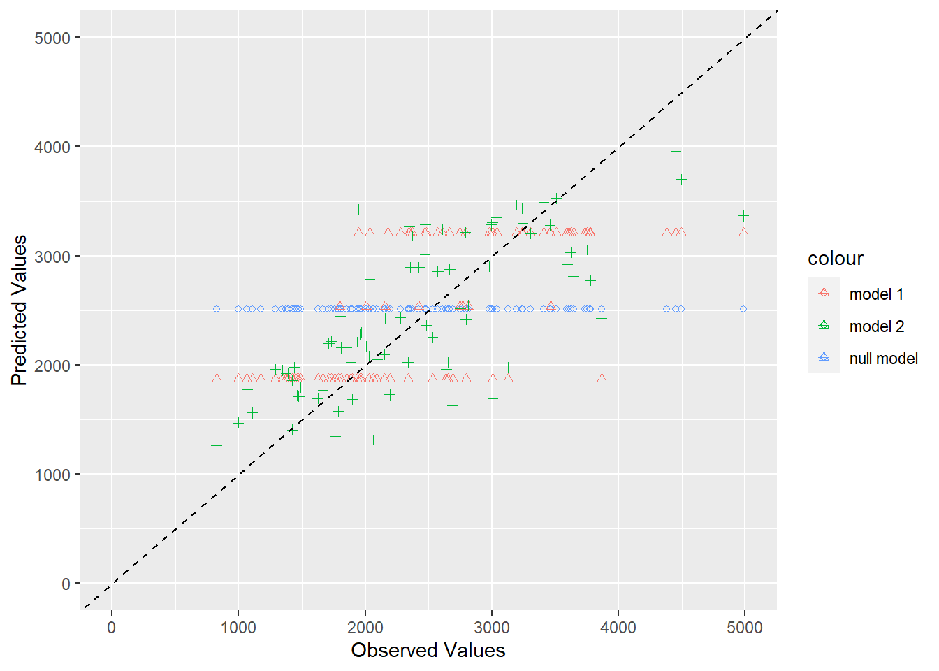
# create a visual representationggplot(plotdata, aes(x = observed)) +geom_point(aes(y = predicted_null, color ="null model"), shape =1) +geom_point(aes(y = predicted_model1, color ="model 1"), shape =2) +geom_point(aes(y = predicted_model2, color ="model 2"), shape =3) +geom_abline(slope =1, intercept =0, linetype ="dashed", color ="black") +#add the 45 degree linexlim(0, 5000) +#limit the x-axis valuesylim(0, 5000) +#limit the y-axis valueslabs(x ="Observed Values", y ="Predicted Values")
The predictions from the null model are a horizontal line because each prediction is just the mean observation. The predictions from model 1 with the DOSE variable only are shown in three horizontal lines, which makes sense because the DOSE variable has 3 discrete values. The predicted values should be the same for each of those 3 dosage values because there are only 3 original values to predict. The predictions for model 2 with all variables is the best and shows a lot of scatter that seems to follow a pattern along the 45 degree line.
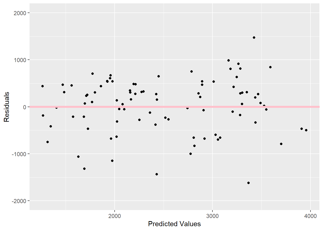
To determine if there is a pattern in the residuals, I will plot the predicted values against the residuals. The formula for finding the residual is just (predicted-observed). I will create a new data frame with the predicted values and residuals first.
# create data frame with predictions and residuals for model 2plotresiduals <-data.frame(predicted_model2 =c(full_aug$.pred), residuals =c(full_aug$.pred - full_aug$Y)) #calculate residuals by predicted - observedplotresiduals
I will plot the new residual values to look for any patterns.
# plot predictions versus residuals for model 2ggplot(plotresiduals, aes(x=predicted_model2, y=residuals)) +geom_point() +geom_abline(slope =0, intercept =0, color ="pink", size =1.5) +#add straight line at 0ylim(-2000,2000) +#make sure y-axis goes the same amount in positive and negative directionlabs(x="Predicted Values", y="Residuals")
Warning: Using `size` aesthetic for lines was deprecated in ggplot2 3.4.0.
ℹ Please use `linewidth` instead.
As Dr. Handel suggested, I see a pattern in these residuals because there are more and higher negative residuals compared to positive residuals. There are 6 observations less than -1000, but there is only 1 observation more than 1000. The positive residuals are grouped together more, while the negative residuals are more spaced out. This could be because there is important information missing or the model is too simple.
Model predictions and uncertainty
To determine uncertainty in the predictions, I will use a bootstrap method to sample the data 100 times and fit the model to each set of predictions.
# set the seed for reproducibilityset.seed(rngseed)# create 100 bootstraps with the training databootstraps <-bootstraps(train_data2, times =100)# create empty vector to store predictions list preds_bs <-vector("list", length =length(bootstraps))# write a loop to fit the model to each bootstrap and make predictionsfor (i in1:length(bootstraps)) { bootstrap_sample <-analysis(bootstraps$splits[[i]]) # isolate the bootstrap sample model <-lm(Y ~ DOSE + AGE + HT + WT + SEX, data = bootstrap_sample) # fit the model using the bootstrap sample predictions <-predict(model, newdata = train_data2) # make predictions with the training data preds_bs[[i]] <- predictions # store predictions in the empty vector}# find an individual bootstrap sample sample <-analysis(bootstraps$splits[[i]])sample
Now that I have all of my predictions stored in a vector, I need to convert it to an array, so I can compute the median and 95% confidence intervals for each one.
# create an empty array to store the predictionsnum_samples <-length(preds_bs)num_datapoints <-length(preds_bs[[1]]) preds_array <-array(NA, dim =c(num_samples, num_datapoints))# fill the array with predictions from bootstrapppingfor (i in1:num_samples) { preds_array[i,] <-unlist(preds_bs[[i]])}# find the median and 95% confidence intervals of each predictionpreds <- preds_array %>%apply(2, quantile, c(0.05, 0.5, 0.95)) %>%t()
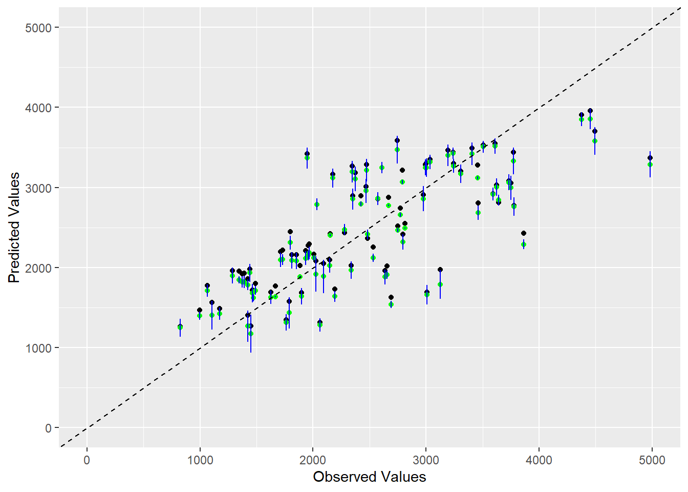
Finally, I will graph the observed values on the x-axis and point estimates from the training data on the y-axis. I will add the median and confidence intervals for the predictions from the bootstrap sampling to the y-axis as well.
# create a data frame with all the necessary variablesfinaldata <-data.frame(observed =c(train_data2$Y), point_estimates =c(full_aug$.pred),medians = preds[, 2],lower_bound = preds[, 1],upper_bound = preds[, 3])# create visualization with all 5 variables ggplot(finaldata, aes(x = observed, y = point_estimates)) +geom_point(color ="black") +geom_point(aes(y = medians), color ="green") +geom_errorbar(aes(ymin = lower_bound, ymax = upper_bound), width =0.1, color ="blue") +geom_abline(slope =1, intercept =0, linetype ="dashed", color ="black") +# add 45 degree linexlim(0, 5000) +ylim(0, 5000) +labs(x ="Observed Values", y ="Predicted Values")
This plot shows that our model does a good job of predicted the observed values because most of the point estimates lie around the 45 degree line. I think some of the variation shown in the bootstrap estimates is accounted for by the fact that the DOSE variable has 3 discrete values, so those predicted values will follow 3 horizontal lines as shown in a previous graph. All of the median values from the bootstrap sampling, shown in green, are father away from the 45 degree line than the actual predicted values, shown in black. There are many instances where the confidence interval from the bootstrapping estimate does not contain the point estimate, but some of the confidence intervals contain the point estimates, especially where the point estimates are clustered. I think this graph is evidence that our model is a decent option for this data because the general pattern of point estimates follows the expected 45 degree line. # Rachel continued this section Now we will use the fitted full model to make predictions for the test data. This will allow us to assess the generalizability of the full model that was fitted. I will start by refitting the full linear regression model to both the training and testing data, using the seed set for the previous analysis.
# predictions based on testing datatest_pred_aug <-augment(full_lmfit, test_data2) %>%# use augment to make predictionsselect(Y, .pred) %>%# select columns for plottingrename(test_pred = .pred) # change the name of the predictions column# predictions based on training datatrain_pred_aug <-augment(full_lmfit, train_data2) %>%select(Y, .pred) %>%rename(train_pred = .pred)# combine prediction columns into one data framecombined_df <-full_join(trial_data5, test_pred_aug, by ="Y") %>%full_join(train_pred_aug, by ="Y") # use full join to retain all values for Y and trial_data 5 for all of the original Y valuesstr(combined_df) # check the structure
'data.frame':   120 obs. of  8 variables:
 $ Y         : num  2691 2639 2150 1789 3126 ...
 $ DOSE      : num  25 25 25 25 25 25 25 25 25 25 ...
 $ AGE       : num  42 24 31 46 41 27 23 20 23 28 ...
 $ SEX       : Factor w/ 2 levels "1","2": 1 1 1 2 2 1 1 1 1 1 ...
 $ WT        : num  94.3 80.4 71.8 77.4 64.3 ...
 $ HT        : num  1.77 1.76 1.81 1.65 1.56 ...
 $ test_pred : num  NA NA NA NA NA NA NA NA NA NA ...
 $ train_pred: num  1628 1962 2097 1576 1976 ...
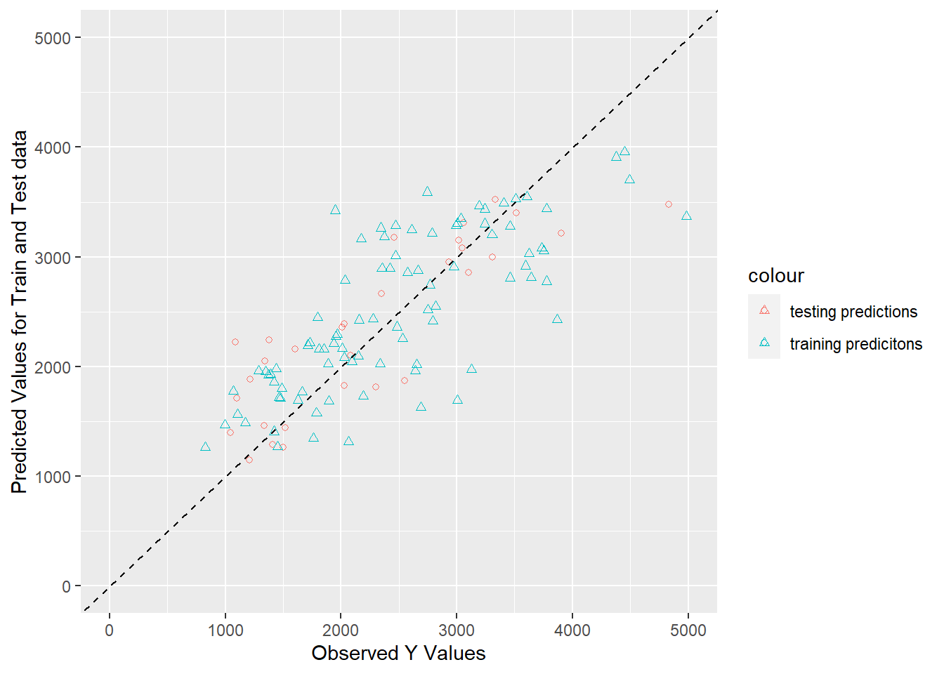
Now, we will plot these two model predictions against the original Y observations to visualize if the testing data produced predictions similar to the training data (and if the model in generalizable).
# grap both predictionstrain_test_plot <-ggplot(combined_df, aes(x = Y)) +geom_point(aes(y = test_pred, color ="testing predictions"), shape =1) +geom_point(aes(y = train_pred, color ="training predicitons"), shape =2) +geom_abline(slope =1, intercept =0, linetype ="dashed", color ="black") +#add the 45 degree linexlim(0, 5000) +#limit the x-axis valuesylim(0, 5000) +#limit the y-axis valueslabs(x ="Observed Y Values", y ="Predicted Values for Train and Test data")print(train_test_plot)
The chart above displays that the training data predictions and testing data predictions follow the same pattern. This means that the model captures the same trends that it did on the testing data as when it was fitted using the training data. This means that the model is generalizable when presented with “new” data. However, the pattern in both sets of predictions shows that a trend was not captured. Even though the model is generalizable, it is also under-fitted and may be too flexible. This means that more tuning, additional predictors, or a larger sample size, will help the model fit the unrepresented trend.
Conclusions
We want to make sure that any model we have performs better than the null model. Is that the case?
According to the RMSE computations for the single predictor model, full model, and null model, which are 560, 520, and 993 respectively, the models including any predictor are both better than the null model. However, we see in the plot of the predicted values of both models versus the null, that the model including the single predictor is not much better than the null model. The null model shows a single horizontal line of predictions, while the single predictor model shows three horizontal lines of predictions. The points in the single predictor model follow the trend (of the 45 degree line) slightly better than the null model, but with only three possible values for the predictor (DOSE), the overall trends of Y are not captured. When you add in all of the predictors, this allows more trends to be captured. This is shown in the graph of the full model predictions, where the points more closely follow the 45 degree trend line.
Does model 1 with only dose in the model improve results over the null model? Do the results make sense? Would you consider this model “usable” for any real purpose?
Model 1 with only DOSE as a predictor slightly improves the results compared to the null model. As discussed before, model 1 has a much lower RMSE value and follows the trend line slightly better than the null model. However, because there are only 3 options for dose, it leaves out many trends contributing the the distribution of Y. This is why the single predictor model would not be usable for any real purpose. Although one could use it to predict the Y given DOSE, we learn that many other predictors impact the trends in Y and DOSE might not be the best predictor.
Does model 2 with all predictors further improve results? Do the results make sense? Would you consider this model “usable” for any real purpose?
Model 2 with all of the predictors does improve the predictions compared to model 1 and the null model. First, the RMSE is lower for the full model than all of the others. Secondly, in the graph, you can see a clear cloud of points following the 45 degree trend line. The full model predictions follow the trend line more closely than all of the other model predictions, showing that the full model fits best. However, there is still a pattern, seen in the residual plot, where higher predicted values are more scattered and contain more outliers. This means that the full model still is not able to capture all of the trends contributing to the observed Y values. This model is still more usable for predicting Y given any of the predictors in the model, because it is more accurate. It must be kept in mind that for larger Y values, the predictive power of the full model likely decreases. This means that it can be used to make predictions for small Y values but not larger ones.